SoftPlus#
The Softplus function is defined as:
Softplus(x) = β * log(1 + exp(β * x))
where:
Softplus is a smooth approximation to the ReLU function and can be used to constrain the output of a machine to always be positive.
For numerical stability, the implementation reverts to the linear function when
input * β > threshold.
Parameters:#
beta(int): The β value for the Softplus formulation. Default: 1.threshold(int): Values above this revert to a linear function. Default: 20.
Implementation#
Piecewise Polynomial approximation (PPA) stands as a computational method for approximating functions, offering a balanced compromise between latency and memory utilization. It involves dividing the input range into K segments, taking into account the \(x_i\) samples within the interval [\(x_L , x_H\)] and the corresponding function values \(f(x_i)\). Within PPA, each of these segments is approximated using a polynomial expression as expressed in following equation:
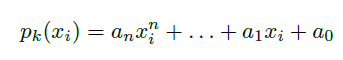
where \(p_k()\) denotes the polynomials corresponding to each segment (k= 1,…K,), \(a_n\) represents the polynomial coefficients, and n denotes the polynomial degree. This approach enables efficient approximation of complex functions by representing them as a combination of simpler polynomial expressions, facilitating adjustable optimization tailored to specific hardware constraints.
More specifically, for the implementation of the Softplus activation function [4] methodology was followed. In [4], a PPA with a wordlength-efficient decoder was employed, which is more improved compared to Simple Canonical Piecewise Linear (SCPWL) and Piecewise Linear Approximation Computation (PLAC) because it optimizes the polynomial indexation.
This approach incorporates adaptive segmentation, polynomial approximation, quantization, and optimization processes which entail to the decrease of hardware resources. Its methodology automatically establishes segment limits based on function slope and user-defined parameters, while it also employs quantization to determine the Fixed-point (FxP) format necessary for achieving the desired accuracy in Signal-to-Quantization Noise Ratio (SQNR).
The evaluation range for this specific AF is [-4,4]. The polynomial coefficients that were calculated using the Vandermonde Matrix [4] are presented in the following table in both float and fixed-point format. It is worth mentioning that the quantization applied to these coefficients is a wordlength of 16 bits, with 15 of those bits representing the fractional part of the number.
Segment Number |
Segment Boundaries |
Format |
a2 |
a1 |
a0 |
|---|---|---|---|---|---|
1 |
[-4, -2) |
Float |
0.0238 |
0.1948 |
0.4184 |
Fixed |
0x030b |
0x18ef |
0x358e |
||
2 |
[-2, 0) |
Float |
0.0969 |
0.472 |
0.68844 |
Fixed |
0x0c67 |
0x3c68 |
0x581e |
||
3 |
[0, 2) |
Float |
0.0969 |
0.528 |
0.68844 |
Fixed |
0x0c67 |
0x4397 |
0x581e |
||
4 |
[2, 4] |
Float |
0.0238 |
0.8052 |
0.4184 |
Fixed |
0x030b |
0x6710 |
0x358e |
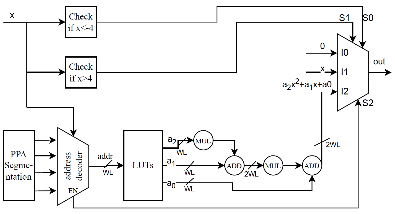
When it comes to the hardware architecture, the High-Level Flow Diagram of Softplus can be seen in the following figure. It initially checks whether the input is in the evaluation boundaries. If it is over the boundaries, then the output will be the input itself, and if it is under the minimum boundary, the result will be 0. When the input is in the region [-4,4], then the PPA has already segmented the boundaries into 4 regions. Depending on the boundary the input lies, the address decoder selects from the LUTs which coefficients will be used. Finally, the output will be a 2nd order polynomial based on the following equation with 15bits of fractional part:
\(p_k(x_i) = a_2 x^2 + a_1 x + a_0\)