Fixed-Point Linear Layer#
The fixed_linear module implements the Pytorch Linear layer. Given the input vector \(x \in \R^{m}\), weights matrix \(W \in \R^{n \times m}\), and bias row vector \(b \in R^n\) where \(m, n\) are the input and output feature counts respectively, fixed_linear returns \(y \in \R^{n}\). For example, taking \(m = n = 4\):
\(y = x W^T + b = \) \( \begin{bmatrix} x_1 & x_2 & x_3 & x_4 \end{bmatrix} \) \( \begin{bmatrix} w_{1, 1} & w_{1, 2} & w_{1, 3} & w_{1, 4} \\ w_{2, 1} & w_{2, 2} & w_{2, 3} & w_{2, 4} \\ w_{3, 1} & w_{3, 2} & w_{3, 3} & w_{3, 4} \\ w_{4, 1} & w_{4, 2} & w_{4, 3} & w_{4, 4} \end{bmatrix} \) + \( \begin{bmatrix} b_1 & b_2 & b_3 & b_4 \end{bmatrix} \) = \( \begin{bmatrix} y_1 & y_2 & y_3 & y_4 \end{bmatrix} \)
Overview#
The fixed_linear module follows the dataflow streaming protocol and works through a sequential dot product operation.
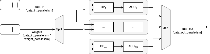
The module has the following parameters, following the hardware metadata standard (see here). Besides PRECISION_DIM_* parameters, which dictate the numerical precision, and TENSOR_SIZE_DIM_*, which is directly inferred from Pytorch tensor shapes, the following parameters can be adjusted to affect hardware performance.
Parameter |
Default Value |
Definition |
|---|---|---|
DATA_IN_0_PARALLELISM_DIM_0 |
4 |
Number of elements per transaction at the input interface. Dictates the number of transactions to compute the full layer. |
WEIGHT_PARALLELISM_DIM_0 |
4 |
Number of columns of the weights matrix per transaction at the weights interface. This is equivalent to the number of dot product modules. Also dictates the number of backpressure cycles on the input interface (see Latency Analysis below) |
DATA_OUT_0_PARALLELISM_DIM_0 |
WEIGHT_PARALLELISM_DIM_0 |
Number of elements per transaction at the output interface. |
BIAS_PARALLELISM_DIM_0 |
WEIGHT_PARALLELISM_DIM_0 |
Number of elements per transaction at the bias interface. Dictates the number of fixed-point adders. |
Example dataflow#
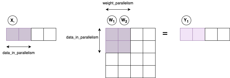
Assume a configuration where DATA_<IN/OUT>_TENSOR_SIZE \(= 4\), DATA_IN_PARALLELISM \(= 2\) and WEIGHT_PARALLELISM \(= 2\). Hence each input data beat has a sub-vector of 2 elements, each weight beat has 4 elements (2 sub-columns of 2 elements) and there are 2 dot product modules. When the first data beat is driven valid, fixed_linear accepts the first weight beat and stalls back the input interface, while driving the dot product modules to compute \(X_1 \cdot W_1\) and \(X_1 \cdot W_2\). This results in partial results for the output sub-vector \(Y_1\).
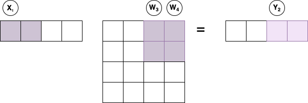
The partial outputs are stored in local registers in the next cycle while \(X_1 \cdot W_3\) and \(A \cdot W_4\) are computed resulting in partial products for the output sub-vector \(Y_2\) and the ready signal is driven for the input data interface.
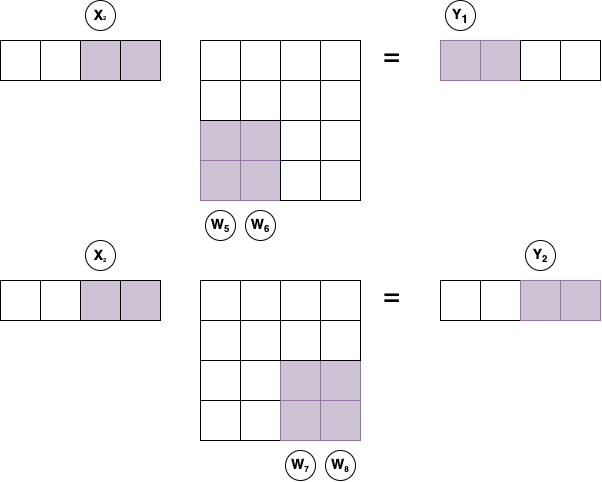
The same process is repeated with the second input sub-vector \(X_2\) and weight sub-columns \(W_{5..8}\). The final output sub-vectors \(Y_1\) and \(Y_2\) are ready and streamed out after the 3rd and 4th cycles, respectively.
Latency Analysis#
The time taken to compute a linear layer using the fixed_linear module, \(L_{FL}\) can be broken down into 2 phases, the input driving phase \(L_L\), and the pipeline unloading phase \(L_U\) that begins after the last input beat is transferred.
When the WEIGHT_PARALLELISM_DIM_0 parameter is set to DATA_OUT_0_TENSOR_SIZE_0, the input tensor can be transferred at full bandwidth, hence \(L_I\) is equivalent to the number of cycles required to transfer the input tensor tensor size in DATA_IN_0_PARALLELISM_DIM_0 sized beats.
\(L_{FL} = L_I + L_U = \frac{\text{DATA_IN_0_TENSOR_SIZE}}{\text{DATA_IN_0_PARALLELISM}} + L_{DP} + L_{ACC}\)
\(L_U\) is equivalent to the propagation latency of a given beat through the dot-product module \(L_{DP}\) and accumulator \(L_{ACC}\), given by the following.
\(L_{DP} = 2 + log_2(\text{DATA_IN_0_PARALLELISM_DIM_0})\)
\(L_{ACC} = 1\)
When \({\text{WEIGHT_PARALLELISM_DIM_0}} < \text{DATA_OUT_0_TENSOR_SIZE\_0}\), the input driving bandwidth is reduced since a number of weight beats are read for each input beat. The input driving phase is scaled by the following factor, leading to the following total latency.
\(L_{FL} = \left(\frac{\text{DATA_IN_0_TENSOR_SIZE}}{\text{DATA_IN_0_PARALLELISM}}\right)\left(\frac{\text{WEIGHT_TENSOR_SIZE}}{\text{WEIGHT_PARALLELISM}}\right) + log_2(\text{DATA_IN_0_PARALLELISM_DIM_0}) + 3\)